Section 5
The final block now opens with unsupervised evaluation and then turns agreement between clustering models into a CLAIRE response matrix.
Associated Notebooks
If you want to run this block locally or in Colab, the sequence is now anchored by:
04_00_unsupervised_evaluation_toy_problems.ipynb, which now serves as the opening bridge inside the CLAIRE block and makes local clustering difficulty visible before any latent fitting happens.05_00_claire.ipynb, which contains the main guided walkthrough for the response-matrix and latent-analysis pipeline.05_01_extra_negative_disc.ipynb, which remains the optional companion notebook for the extra analysis linked from this section.05_02_activities.ipynb, which is the main participant activity for the final block.
All of these notebooks can use the shared helpers from utils/handson.py and utils/transform.py.
The final block now starts from unsupervised evaluation
Clustering is often introduced through aggregate metrics, and that is still a useful starting point. But once the geometry becomes nontrivial, a single score can hide that some instances are easy, some are ambiguous, and some are especially informative because they concentrate disagreement.
That is why the CLAIRE block now begins here rather than in a separate standalone section. Before agreement becomes a response matrix, the room first needs to see that disagreement is already a meaningful signal about the dataset itself.
A clean baseline shows when averages are enough
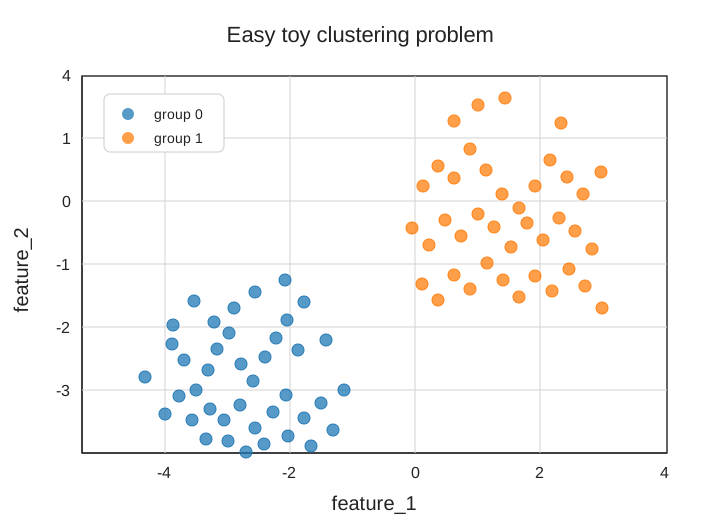
We begin with an easy toy problem. The two groups are compact, well separated, and visually stable. In that setting, different clustering models have very little room to disagree in a meaningful way.
| Model | ARI | Silhouette | Calinski-Harabasz | Davies-Bouldin |
|---|---|---|---|---|
| Agglomerative | 1.000 | 0.767 | 2308.063 | 0.329 |
| K-means | 1.000 | 0.767 | 2308.063 | 0.329 |
| Spectral | 1.000 | 0.767 | 2308.063 | 0.329 |
This table is useful precisely because it is boring. The models agree, the metrics agree, and no local difficulty story is being hidden. That baseline matters because it makes the next shift much easier to read.
Harder geometry makes disagreement informative
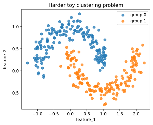
The next step is to move to a harder geometric structure. The data are still interpretable, but now the groups are curved and local ambiguity matters much more.
| Model | ARI | Silhouette | Calinski-Harabasz | Davies-Bouldin |
|---|---|---|---|---|
| Spectral | 0.722 | 0.398 | 299.124 | 0.930 |
| K-means | 0.235 | 0.485 | 472.211 | 0.773 |
| Agglomerative | 0.194 | 0.476 | 453.296 | 0.776 |
At this point, the evaluation story stops being uniform. Spectral clustering is strongest under ARI because it stays closer to the teaching labels, while K-means and agglomerative clustering look more favorable under compactness-oriented metrics. The question is no longer just which number is highest. The question becomes which structural property each metric is rewarding and where that reward is coming from.
Agreement already reveals where the hard instances live
The bridge notebook answers that question by estimating difficulty through agreement across clustering models. If the models treat an instance consistently, the instance is easier. If they diverge on it, the instance is harder.
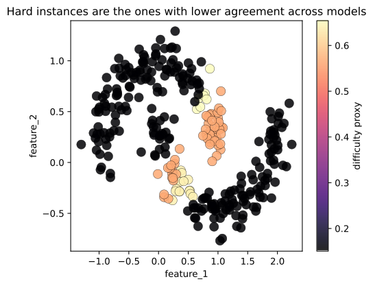
This is the key conceptual handoff into CLAIRE. Before any latent model is fitted, the room has already seen that agreement is not just a side effect of model comparison. It is evidence about which parts of the dataset are structurally easy, difficult, or ambiguous.
From disagreement to a response matrix
CLAIRE takes that agreement signal and turns it into data. Instead of recording whether a model is correct on an item, it records how strongly that model agrees with the rest of the pool on a given instance.
Formally, let P = {pij}M x N denote the response matrix, with M clustering models and N instances. Each entry pij is the normalized agreement of model i on instance j. For another model i’ != i and another instance j’ != j, the agreement indicator is
\[c_{i,i'}^{j,j'} = \begin{cases} 1, & \text{if models } i \text{ and } i' \text{ agree about whether instances } j \text{ and } j' \text{ belong together or apart}, \\ 0, & \text{otherwise}. \end{cases}\]and the CLAIRE response is
\[p_{ij} = \frac{1}{(M-1)(N-1)} \sum_{i' \neq i} \sum_{j' \neq j} c_{i,i'}^{j,j'}.\]In the workshop code, that construction is carried out by TransformPairwise before Beta4 is fitted. The response matrix does not preserve every detail of the original partitions, but it does preserve a normalized view of how each model agrees with the rest of the pool around each instance. That is exactly what allows the method to connect clustering geometry to latent item analysis.
The CLAIRE toy problem keeps the workflow readable
The guided notebook starts from a three-cluster toy problem so the room can read the geometry before any latent fitting happens.
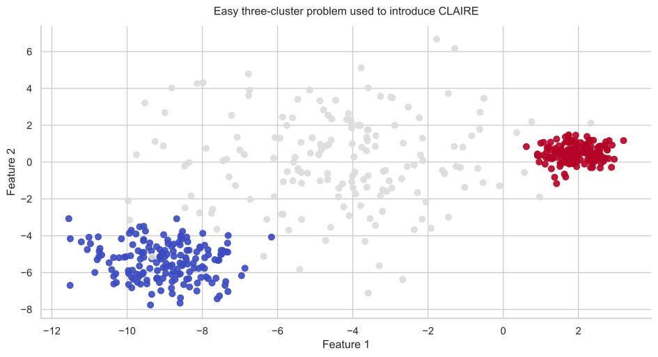
This choice is pedagogically important. By this point the audience is already carrying the unsupervised intuition from the bridge notebook, so the main CLAIRE walkthrough can focus on the transformation itself: dataset, model pool, partitions, agreement matrix, latent fit, interpretation.
Latent ability is related to, but not reducible to, classical metrics
Once the agreement matrix is fitted with Beta4, the notebook compares the resulting latent abilities with familiar clustering metrics.
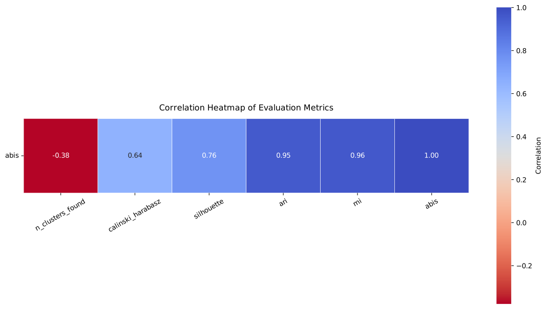
This protects the method from a common misunderstanding. CLAIRE ability is not merely an average agreement score disguised as a latent parameter. The correlations with classical metrics are meaningful, but they do not reduce the latent quantity to any single traditional summary.
Difficulty and discrimination become geometric again
The next step places the latent quantities back on the dataset. Instances are colored by difficulty and sized by discrimination, so the geometry becomes a latent landscape rather than a single average score.
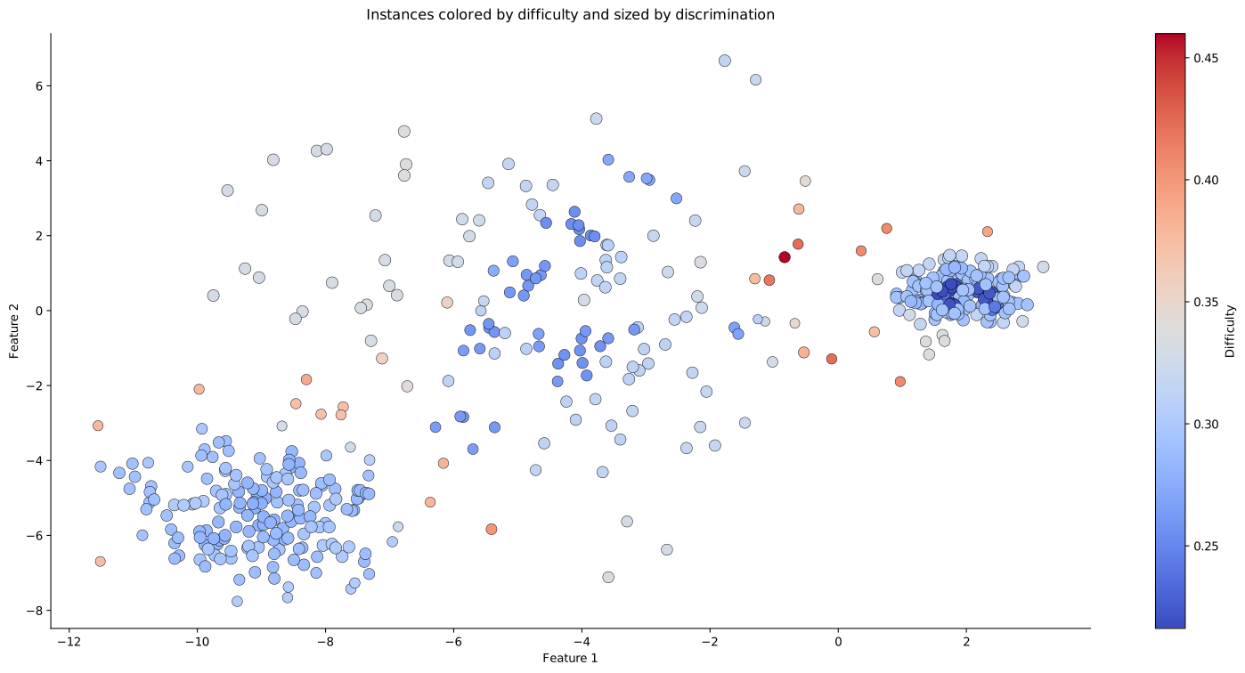
This is where the whole workshop closes the loop. The supervised block taught the room to care about local difficulty. The unsupervised bridge taught the room to read disagreement as a local signal. CLAIRE now turns that same local signal into a latent analysis where difficulty and discrimination can be read back onto the geometry.
The easiest and hardest instances still induce different curves
The guided notebook closes the main CLAIRE path by comparing the response curves of the easiest and most difficult instances.
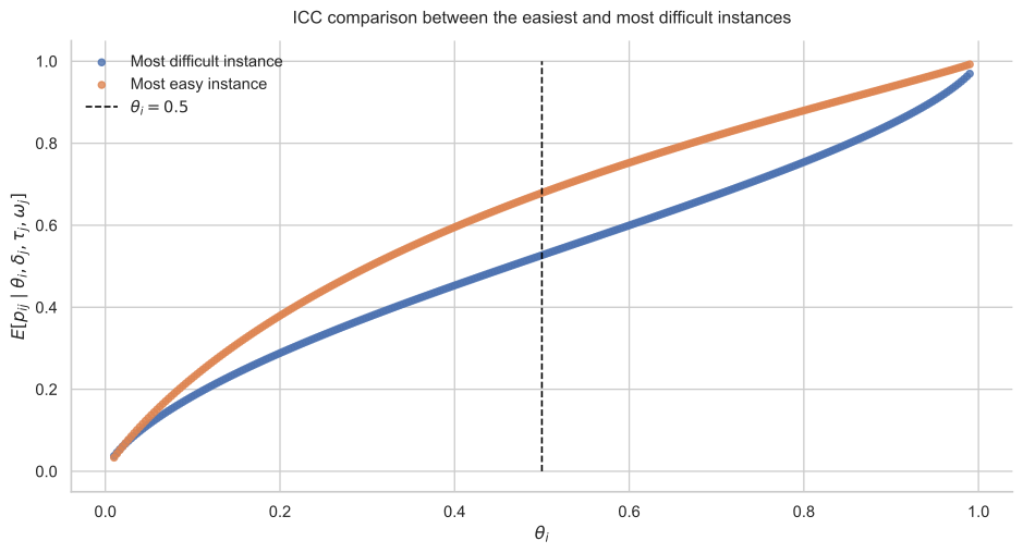
After all the machinery of partitions, pairwise agreement, and response-matrix construction, the workshop comes back to a familiar visual language: curves. That return matters because it shows that the latent interpretation is not just numerical bookkeeping. It is changing how we read the response behavior of individual instances.
Why CLAIRE now closes the workshop by itself
The final block ends here because CLAIRE depends on everything that came before. The supervised section taught the room to care about local difficulty. Binary IRT taught the language of ability, difficulty, and discrimination. Beta4 showed that bounded responses can still support that language. The unsupervised bridge made agreement visible as a meaningful signal. CLAIRE is where those pieces finally become one workflow.
Questions for Discussion
- Why is agreement a more interesting signal than correctness in this setting?
- What does the response matrix keep from the clustering geometry and what does it discard?
- Why is latent ability different from simply averaging agreement across items?
- What does the unsupervised bridge add before the CLAIRE fitting step even begins?