Section 3
The third section keeps the latent IRT logic but moves from binary outcomes to bounded responses and richer discrimination behavior.
Associated Notebook
If you want to run this overview locally or in Colab, the associated guided notebook is:
03_00_beta4_irt.ipynb, which introduces the Beta4 parameterization, curve family, and recovery logic used in this section.
The local notebook environment can also import the shared helpers from utils/handson.py and utils/transform.py.
From binary IRT to bounded responses
The previous section introduced latent ability, item difficulty, and item discrimination in a binary setting. Beta4-IRT keeps that latent interpretation, but it moves to responses that live on a bounded interval instead of being restricted to success or failure.
This matters because many evaluation signals are not naturally binary. Agreement proportions, bounded scores, and normalized response intensities all call for a model that can live on (0, 1) without abandoning the interpretability of latent ability and item parameters. In other words, the question is no longer just whether a respondent succeeded. The question becomes how strongly a bounded response reflects latent ability and item structure.
Beta4 as an adaptation of Beta3
The missing formal bridge is important here: Beta4-IRT is introduced as an adaptation of Beta3-IRT. Before the expected response, Beta3 defines the bounded response and its latent parameters as:
\[p_{ij} \sim \mathcal{B}(\alpha_{ij}, \beta_{ij}),\] \[\alpha_{ij} = \left(\frac{\theta_i}{\delta_j}\right)^{a_j}, \qquad \beta_{ij} = \left(\frac{1-\theta_i}{1-\delta_j}\right)^{a_j},\] \[\theta_i \sim \mathcal{B}(1,1), \qquad \delta_j \sim \mathcal{B}(1,1), \qquad a_j \sim \mathcal{N}(1,\sigma_0^2).\]With those definitions in place, the equation bellow writes the expected bounded response with a single discrimination parameter $a_j$:
\[E[p_{ij} \mid \theta_i, \delta_j, a_j] = \frac{\alpha_{ij}}{\alpha_{ij} + \beta_{ij}} = \frac{1}{1 + \left(\frac{\delta_j}{1-\delta_j}\right)^{a_j} \left(\frac{\theta_i}{1-\theta_i}\right)^{-a_j}}.\]Beta4 keeps the same bounded-response logic, but rewrites discrimination as two separate terms so that sign and magnitude can be modeled explicitly. In Equation bellow, using $\tau_j$ for the sign component and $\omega_j$ for the magnitude component, the expected response becomes:
\[E[p_{ij} \mid \theta_i, \delta_j, \omega_j, \tau_j] = \frac{1}{1 + \left(\frac{\delta_j}{1-\delta_j}\right)^{\tau_j \cdot \omega_j} \left(\frac{\theta_i}{1-\theta_i}\right)^{-\tau_j \cdot \omega_j}}.\]So the conceptual move from Beta3 to Beta4 is compact but meaningful: instead of using one single $a_j$, Beta4 decomposes the effective discrimination into sign and magnitude. That is what lets the model represent richer item behavior while preserving the same latent reading of ability and difficulty.
Beta4 curves can express richer behavior
The notebook begins with a compact item bank where difficulty is still bounded in (0,1), but discrimination is decomposed into sign and magnitude before being interpreted through the product $\tau_j \omega_j$.
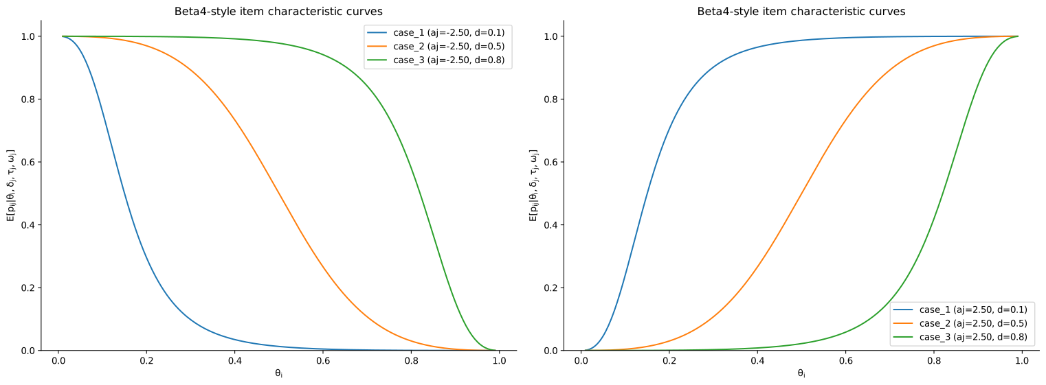
This plot is the visual entrance to Beta4. It tells the audience that bounded responses need more expressive curves than the standard binary logistic family. The familiar IRT story is still present, but the model is no longer limited to one rigid response shape. That extra flexibility is what makes Beta4 useful for agreement scores, proportions, and other bounded evaluations that are too rich to be reduced to simple 0/1 outcomes.
The important point is not just that the shapes look different. The important point is that the interpretive language survives the generalization. We still want to talk about who is strong, which items are hard, and which items separate respondents well. Beta4 extends the response family without giving up that latent-reading discipline.
The synthetic experiment declares the generating distributions explicitly
Before any fitting happens, the notebook samples latent quantities from known distributions:
\[\theta_i \sim \mathrm{Beta}(1, 1), \qquad \delta_j \sim \mathrm{Beta}(1, 1), \qquad a_j \sim \mathcal{N}(1, \sigma_0^2).\]The point is not to trust the fitted parameters abstractly. The point is to compare the fitted quantities against the generating ones and verify that the model is recovering a meaningful latent structure. This is one of the most important habits in the whole workshop: when a latent model becomes richer, we should become more demanding about whether its parameters can be read sensibly.
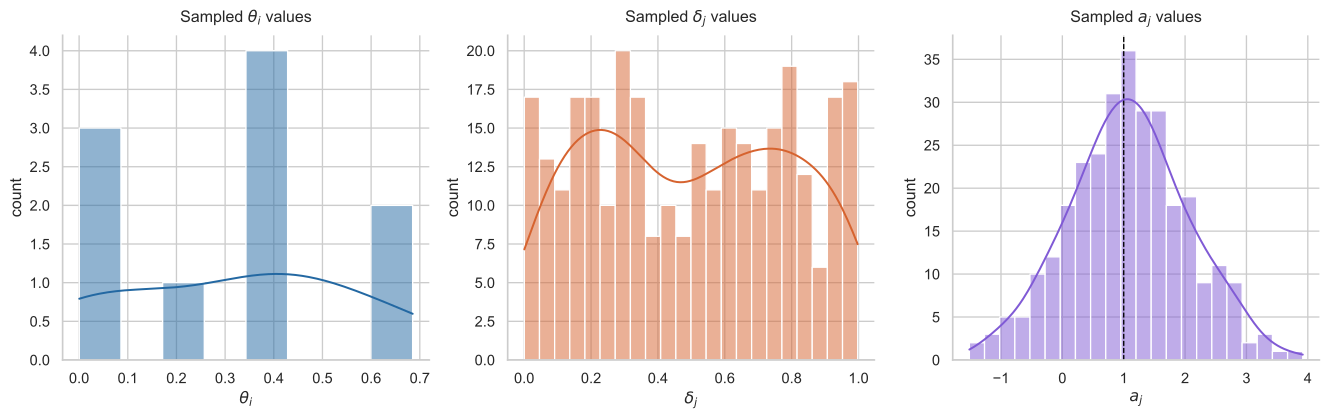
Those distributions matter because they define the world from which the responses are created. The recovery exercise is therefore not just a fitting exercise. It is a test of whether the model can rediscover the latent organization that actually produced the data.
Recovery is what turns flexibility into trust
Once the bounded responses are generated, the notebook fits Beta4 and compares estimated quantities with the generating ones.
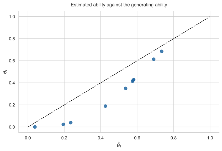
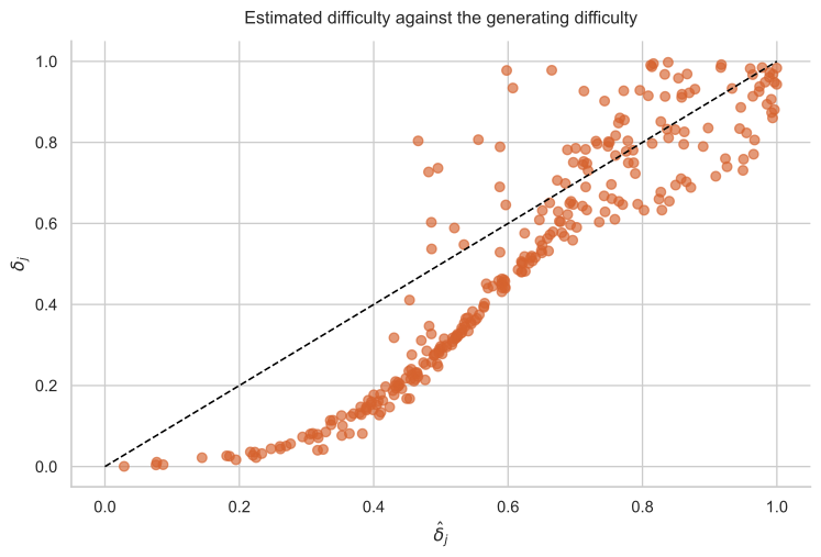
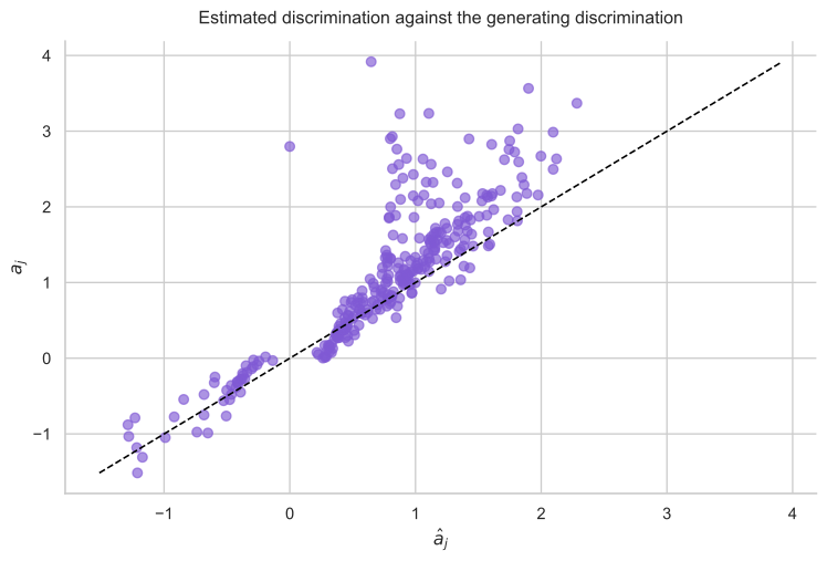
These plots are central because they answer the natural skepticism the audience should have: if the model is more flexible, are the fitted parameters still meaningful? The recovery story is the answer. Ability and difficulty should track the generating values closely if the latent interpretation is stable. Discrimination is usually the hardest quantity to interpret visually, so the recovery plot for $a_j$ becomes especially important. It shows that the model is not simply fitting arbitrary bounded curves. It is recovering a structured latent description.
Why this section has to come before CLAIRE
Beta4-IRT should be understood before the workshop turns to agreement-based evaluation. Once the room sees that Beta4 can recover ability, difficulty, and discrimination from bounded synthetic responses, the later CLAIRE workflow becomes much easier to motivate. The response matrix may change in Section 5, but the latent interpretation is already in place here.
This is the strategic role of the section. Beta4 is the bridge between classical IRT and the more unusual response construction that CLAIRE will later introduce. Without this section, CLAIRE could look like two difficult ideas at once: a new response matrix and a new latent model. With this section in place, only the response matrix is new; the latent model has already been read and trusted.
Questions for Discussion
- What does Beta4 preserve from binary IRT and what does it generalize?
- Why is it important to inspect generating and fitted parameters side by side?
- Which parameter is hardest to interpret visually, and why?
- Why should the room understand Beta4 before moving to CLAIRE?